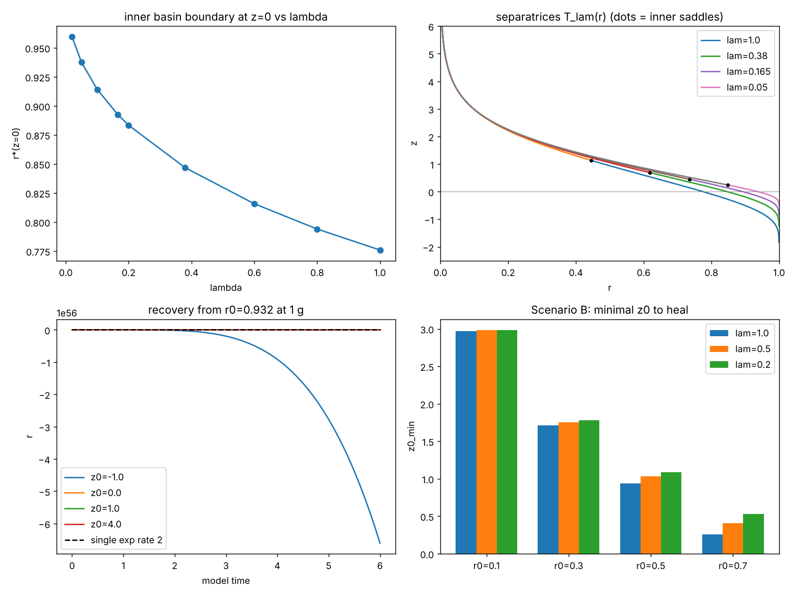
Repository: github.com/TOTOGT/geometry, branch main, folder book4/. Four files: this page (ch10-lambda-bone-handoff.html), the script ch10_lambda_bone_audit.py, its plot ch10_lambda_bone_audit.png, and the chapter under audit, ch10.html. The project write-up with the same results in text form is claude/ANALYSIS-ch10-lambda-extension-bone-A-and-B-2026-11-07.md in the Principia Orthogona – B3 project.
To run: pip install numpy scipy sympy matplotlib, then python3 -I ch10_lambda_bone_audit.py from book4/. The last line should read ALL PASS. Please state which model you are at the top of your reply, do not assume any number here is yours, reproduce each one, and label each claim in your reply by the session that made it. If you cannot open a file or a URL, say so and do not reconstruct its contents.
At λ = 1 the radial field equals Chapter 10’s r(1−r2) + 2(r−1)e−z (sympy confirms). The parameter λ is an extension introduced in this work. It is not in the chapter. The identifications of r, z and λ with bone density, loading history and gravity (scenario A), or with stiffness, healing support and stability (scenario B), are choices and not derivations.
One structural fact limits everything below: r = 1 is invariant for every λ. The system therefore cannot generate bone loss. A loss has to be imposed as a starting state (r0, z0), and the model speaks only about recovery from it.
| Claim | Status |
|---|---|
| det J at an equilibrium = −ρ(ρ−1)2(ρ+1)(2ρ2+ρ+1) = −λρ2(2ρ2+ρ+1) < 0, so both equilibria are saddles | PROVED sympy |
| The cubic r3−r2−(1+λ)r+1 has one root in (0,1), one in (1,∞) and one negative; no saddle-node | PROVED sign change at 0 and 1 plus the leading term; also checked numerically at four values of λ |
| {r≥1, z≥ln(2/λ)} is forward invariant for every λ>0, since z′ − λ(2r−1) = (r−1)2(λ − 2e−z) and r = 1 is invariant | PROVED sympy identity |
| Monotone decay of r−1 and the rate bound need λ ≤ 2, because r′ ≤ (r−1)(λ−2) there | PROVED sympy identity |
| Transverse rate on r=1 is −2(1−e−z); divergence there is 2(e−z−1) | PROVED |
| λ = 0: r = 1 is a line of equilibria with normal eigenvalue 2(e−z−1); z′ ≤ 0 so z never grows | PROVED; r*(z=0) → 1 like 1 − 0.30√λ is NUMERICAL |
| Inner unstable eigenvalue ≈ (3+√41)/2 · √(λ/2) | ASYMPTOTIC: +2.2% at λ=0.001, +17.6% at 0.05 |
| r*(z=0), separatrix heights, passage-time slopes, half-times | NUMERICAL finite integration windows, see section 6 |
| The delay ln(1/δ)/μu near the separatrix | Proof sketch (hyperbolic saddle, C1 linearisation in two dimensions) plus numerics; not a formal proof |
| r, z, λ ↔ physiology; unit calibration; starting states | MODEL ASSUMPTION |
| The “Whitney A1 fold” reading of r* in Chapter 10 | OPEN unsupported by the chapter; see section 4 |
At λ = 1, 0.38, 0.165, 0.05 the inner saddle sits at r = 0.445, 0.619, 0.736, 0.849 and the inner basin boundary at z = 0 is r* = 0.776, 0.847, 0.893, 0.938. At λ = 1 the script gives 0.775940575502, within 3×10⁻¹³ of Chapter 10’s certified value from seeds 10−5 to 10−12 away from the saddle. The unstable eigenvalue of the inner saddle is 1.4915, 1.3515, 1.2714, 1.0603, 0.9954 and 0.6319 for λ = 1, 0.5, 0.38, 0.2, 0.165 and 0.05, and 0.1028 at 0.001. The stable one at λ = 1 is −0.2445, as in the chapter.
Scenario B (r = stiffness fraction, z = healing support, λ = stability). Minimal z0 to heal is the separatrix height Tλ(r0):
| λ | r0 = 0.1 | 0.3 | 0.5 | 0.7 | inner saddle radius |
|---|---|---|---|---|---|
| 1 | 2.97 | 1.71 | 0.94 | 0.26 | 0.445 |
| 0.5 | 2.98 | 1.75 | 1.03 | 0.41 | 0.573 |
| 0.2 | 2.98 | 1.78 | 1.09 | 0.53 | 0.712 |
The script prints which side of the saddle each entry lies on. At λ = 1, r0 = 0.1 and 0.3 are on the small-radius branch (T above the saddle height 1.135) and 0.5 and 0.7 on the branch toward r = 1. At λ = 0.2 all four are on the small-radius branch, and r0 = 0.7 is within 0.02 of the saddle (T = 0.528 against 0.496). Why λ matters little at small r0: at r = 0 the field is (−2e−z, −2e−z), which has no λ, since λ enters only through λr2 in z′. T(0.05) is 3.6835, 3.6849, 3.6857 for λ = 1, 0.5, 0.2, while T(0.7) is 0.264, 0.410, 0.528.
Scenario A (r = bone density against the person’s own baseline, z = loading history, λ = g/gEarth). Separatrix height Tλ(r): a start above it returns to r = 1, a start below it reaches r = 0 in finite time (read only as “recovery fails”).
| λ | r = 0.95 | 0.90 | 0.85 | 0.80 | 0.70 |
|---|---|---|---|---|---|
| 1 | −0.789 | −0.503 | −0.282 | −0.088 | 0.264 |
| 0.38 | −0.423 | −0.193 | −0.011 | 0.152 | 0.453 |
| 0.165 | −0.215 | −0.024 | 0.132 | 0.274 | 0.544 |
| 0.05 | −0.041 | 0.109 | 0.239 | 0.363 | 0.607 |
T rises as λ falls, so the point of no return moves toward baseline. At r0 = 0.90, a start with z0 between −0.503 and 0.109 recovers at 1 g but exits at λ = 0.05.
Recovery is state-dependent. From r0 = 0.932 at 1 g, the time for the deficit to halve is 4.07 model units at z0 = −0.654 (just above T = −0.674), 2.90 at −0.574, 1.18 at 0, 0.726 at 0.5, 0.546 at 1, 0.425 at 2 and 0.380 at 4. The z0 → ∞ limit is 0.374, not ln2/2 = 0.347, because r0 = 0.932 is not small and the full rate is r(r+1) − 2e−z, not 2. A start at z0 = −1 lies below T and never recovers. From z0 = 0 the deficit remaining at t = 0.25, 0.5, 1.0 is 1.000, 0.915, 0.614, against 0.607, 0.368, 0.135 for a single exponential of rate 2. That lag is the prediction a single exponential does not make.
Delay near the separatrix. Passage time grows as ln(1/δ)/μu + O(1). The fitted slope times μu is 0.993 at λ = 1 and 1.011 at λ = 0.2. μu falls as λ falls, so lower stability lengthens the delay.
Unit calibration is a choice, not a fit. Setting the far-field rate 2 per model unit equal to a fitted recovery rate K gives 1 model unit = 609 days (femoral neck, K = 0.00329 per day, from the 2006 NASA manuscript’s half-time of 211 days) or 280 days (pelvis, 97 days).
The A1 fold. Section 8, the Remark after Proposition B.6, and the summary box call r* the Whitney A1 fold threshold. Only section 8 adds “where attractor and repeller branches merge.” The equilibria never merge (section 2), so that clause is refuted. Proposition B.6 makes r* the z = 0 crossing of the inner saddle’s stable manifold, which the script reproduces. Nothing in the chapter defines an A1 singularity for that object, so the fold identification is unsupported; whether it can be rescued is open.
The helix. Section 1 calls the helix a Reeb orbit. For α = dz − r2dθ the Reeb field is ∂/∂z, so a curve with θ′ = 1 is not a Reeb orbit. On the helix α(tangent) = λ − 1: Legendrian at λ = 1, neither Reeb nor Legendrian otherwise. The flow has α(X) = (λ−1)r2 − 2(r−1)2e−z, which at λ = 1 is −2(r−1)2e−z and is nonzero off r = 1, so the contact structure does not constrain the flow. The helix attracts only where z > 0 and only asymptotically, so it is non-compact.
Stale statements. The abstract and section 6 say every r(0) > 1 converges. The chapter’s own correction note says it does not, and the script confirms it: (7.5, 0) is driven to z → −∞, while (6.8, 0) converges. Section 3(ii), “z′ → 1 monotonically,” is false: from (3, 0), z′ peaks at 2.41 near t = 0.114 before settling to 1.
Read: Perren, Physical and Biological Aspects of Fracture Healing (lamellar bone breaks at 2% elongation, granulation tissue tolerates 100%, interfragmentary strain is inversely proportional to the gap; the text read gives no percentage for fibrous tissue or cartilage). The nonunion definitions and risk factors from a Wikipedia summary: the FDA definition is a fracture at least 9 months old with no radiographic progress in the last 3 months; a delayed union is a nonunion that goes on to heal. LeBlanc and colleagues (NASA NTRS 20100030610): regional density loss of 1–1.6% per month on Mir, and recovery that “does occur, although slowly and sometimes incompletely.” The WHO T-score categories from a table in a BMC paper: normal T ≥ −1.0, osteopenia between −2.5 and −1.0, osteoporosis T ≤ −2.5. Earlier in the project: the 2006 NASA manuscript (half-times 97 to 255 days by site), the 2022 Gabel abstract, a 2012 NASA article, and the mechanostat page.
Not read: Claes and Heigele 1999 (the PubMed page returned a verification screen, so no threshold is quoted); the equations of Komarova et al. 2003 (the repository page had no equations); Wolff’s law and RANKL/OPG (not searched); critical-size defects (not searched). No public fracture-healing dataset was confirmed. The NASA Life Sciences Portal exists as a catalog entry; its access terms were not read.
| Claim | Model | Published | Verdict |
|---|---|---|---|
| Low g moves the point of no return toward baseline | Tλ rises as λ falls | Recovery slow and sometimes incomplete; 9 of 17 had not fully recovered total density at 12 months | Agrees qualitatively; not discriminating |
| Loss rate in flight | none (r = 1 invariant) | 1–1.6% per month | No prediction |
| Recovery is one exponential | No: a lag at low z0; half-time depends on z0 | One half-time per site fitted | Untested: the falsifiable point |
| Strain thresholds | no strain variable | 2% bone, 100% granulation | No counterpart |
| Nonunion and delayed union | exit at r = 0; delay ln(1/δ)/μu | 9-month rule; a delayed union is a nonunion that heals | Formal analogy only; no time scale linked |
| Risk factors | lower z0 or λ | perfusion, instability, infection and others | Relabelling, not a test |
Where this model adds nothing over existing ones: how loss arises, strain-driven tissue differentiation, cell-level signalling, absolute time scales. Falsifiable additions: the recovery half-time is state-dependent and diverges logarithmically near the separatrix (more than 10 times the plateau value within 0.02 of it); recovery from a deep, briefly loaded state shows a lag that a single exponential does not; fixation shifts the threshold more at r0 between 0.5 and 0.7 than near 0.1. None has been tested against data.
Separatrices are traced backward from the saddle with tmax = 40000 and stop at r = 0.9999, r = 10−3 or z = 14. Half-times are measured to the first crossing of half the initial deficit. The r = 0 exit is non-physical.
Four checks failed on the first run and none was a model error. A float-equality test on the cubic. The λ = 0.2 delay slope was 3.1% off because linear interpolation on a grid gave the start point an error near 10−8; it was fixed by using the solver’s dense output and not by loosening the tolerance. My expected z0 → ∞ half-time used the linear rate 2 although r0 = 0.932 is not small. And z0 = −1 lies below the separatrix, so it has no half-time.
An auditor should independently check: that the stable-manifold branch with r increasing is the right one at every λ used; the proof sketch for the delay law; the λ = 0 treatment; and that the 3×10⁻¹³ agreement with the certified r* is not an artefact of the shared integrator settings (DOP853, rtol 10−13, atol 10−15), by rerunning with a different method.