Principia Orthogona · Book 6 · Behavioral Finance · Working Paper

The Forced Urgency Gap

why "selling at a loss" is not identified as a preference, why small liquidity shortfalls cascade, and who collects each and every time — with the extension past Genesove–Mayer and Piketty

Prospect theory locates the pathology of selling in the seller's value function. This paper locates it in the seller's balance sheet. The distinction is not semantic: one diagnosis prescribes investor education, the other prescribes bridge liquidity, and only one of them moved markets when tested at scale (§5). The gap is a single missing state variable — urgency, the shadow price λ on the constraint liquidity escaped; now I need that money — and restoring it reorganizes the identification, the amplification, the distribution, and the recruitment of the losses.

The demand side, from the desk A former registered representative can state it in one sentence: every client wants the best possible return, in the fastest possible time, with as little as possible risk. No asset satisfies this trinity. What the industry supplies instead are payoff shapes that appear to satisfy it — frequent small wins, rare catastrophic losses — and those contracts are precisely the machinery of §3 and §4 below.

§1 · The model in one paragraph

Agents with standard preferences (no kink, no reference point) hold an asset, carry a non-deferrable commitment c̄ (rent, mortgage, food) with default cost χ (eviction, foreclosure), and face an income shock with probability f. Urgency is the Lagrange multiplier λⁱ ≥ 0 on the liquidity constraint; it is strictly positive when cash + income + credit < c̄. A forced sale is a sale at λ > 0 that would not occur at λ = 0 holding beliefs and preferences fixed. Proposition 1: a constrained agent optimally sells at any positive price, including below basis and below fundamental value — the realized loss carries zero information about preferences. It is a statement about the constraint set.

§2 · Theorem 1 — Misattribution

Theorem 1 (non-identification) On data of trades, prices, and paper gains/losses with the liquidity state latent, prospect theory (PT) and standard-preferences-plus-liquidity-constraint (LC) are observationally equivalent in crisis states. Income shocks correlate with drawdowns, so forced sales cluster in the loss domain; a fitted reference-dependent kink absorbs that clustering as spurious loss aversion λ̂_PT > 1. The preference parameter is not identified without observing λ. Identification requires an instrument shifting the liquidity state independently of returns — and the two available natural experiments both reject the preference-only model (§5).

§3 · Theorem 2 — The cascade, and the $750 seed

Market clearing with limited arbitrage gives p = μ − κS; lower prices tighten collateral, margin, and refinancing constraints, so forced supply S depends on price. With feedback coefficient ρ = κ|∂S/∂p|, losses amplify by A = 1/(1−ρ), diverging as ρ → 1, with discontinuous fire-sale equilibria beyond a threshold. The total mark-to-market loss is borne by all holders, not only the shocked fraction f.

Corollary — the $750 → ten-percent-of-America corollary An ex-ante transfer of the minimal shortfall (order $10²–$10³ per household: median eviction arrears, one bridged mortgage payment) sets forced supply to zero and prevents A-multiplied losses. Literature ballparks: ~27% forced-sale discount and ~1% spillover per nearby foreclosure (Campbell–Giglio–Pathak 2011); ~$78k all-in social cost per foreclosure (JEC 2007); peak distress ~1 in 10 U.S. mortgages (2010). The cascade-cost-to-shortfall ratio is order 10² per event before spillovers. The amplification is the crisis; the shortfall is merely its seed. A PT operator prescribes "don't panic" education, which moves λ not at all; the constraint model prescribes bridge liquidity at cost T with effect A·T. Misattribution aims policy at the wrong variable.

§4 · Who collects, and how the harvested are recruited

In the fire-sale equilibrium, permanent-capital buyers — lockup vehicles, corporate balance sheets, institutional single-family-rental platforms — buy at the discount and earn it as rent for supplying liquidity-immunity. Every uninsured cycle is a wealth transfer from urgent to non-urgent balance sheets. Because that rent is increasing in system fragility (∂rent/∂ρ > 0), the harvesting side rationally opposes the cheap intervention — not from malice, but because bridge liquidity destroys the discount it harvests. Iterated, this is a concentration ratchet: each crash moves stock from constrained households to permanent capital, enlarging its absorption capacity and its stake in the next crash. The post-2008 institutional SFR wave is one realized iteration.

Proposition 2 — the manufacturing channel The two named behaviors are not rivals; they are a production chain. The loss-averse client demands loss-capping contracts — stop losses, margin, guarantees, on-demand redemption — and each converts the soft preference "I don't want losses" into the hard constraint "I must sell at p ≤ p^stop." Stop-loss mass raises forced supply and its price-sensitivity, hence ρ and A. The disposition effect governs the quiet regime (holding losers, capping winners); the contracts it demands create the loud regime (cascades of triggered sales). The systematic trader capping gains at +1% with stops underneath has engineered negative skew, contractual membership in the cascade, and the counterparty seat the permanent-capital buyer is waiting for — recruited voluntarily, by his own loss aversion. The only achievable form of "never lose" is never realizing at the bottom: funding that cannot be called, obligations covered without touching the portfolio, no contract converting a price into a mandatory sale.

§5 · Macro evidence, 1971–2026

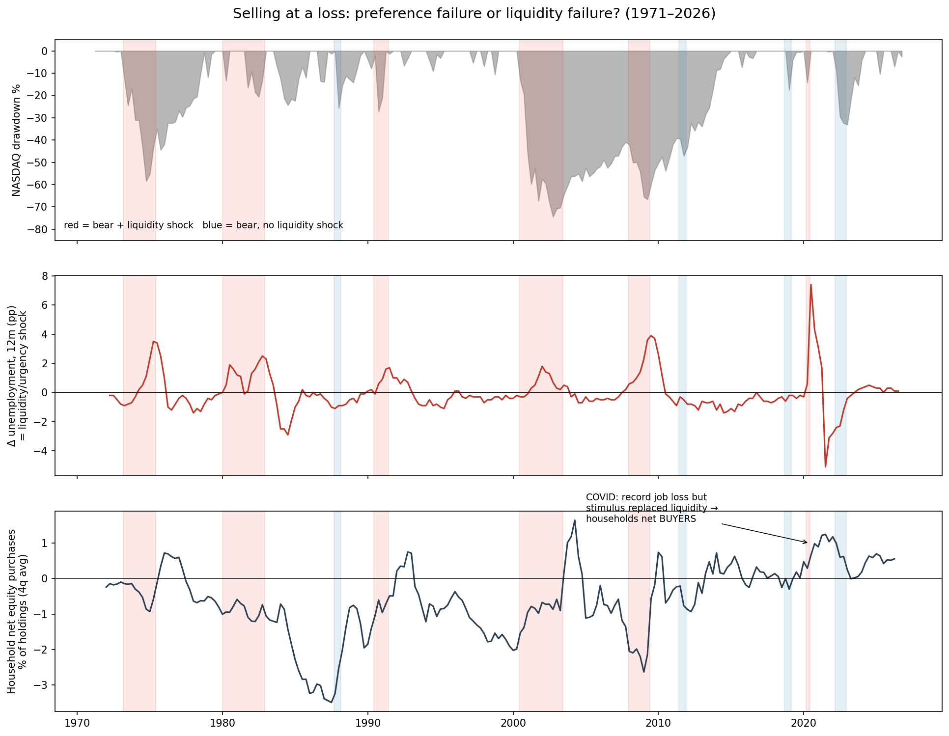
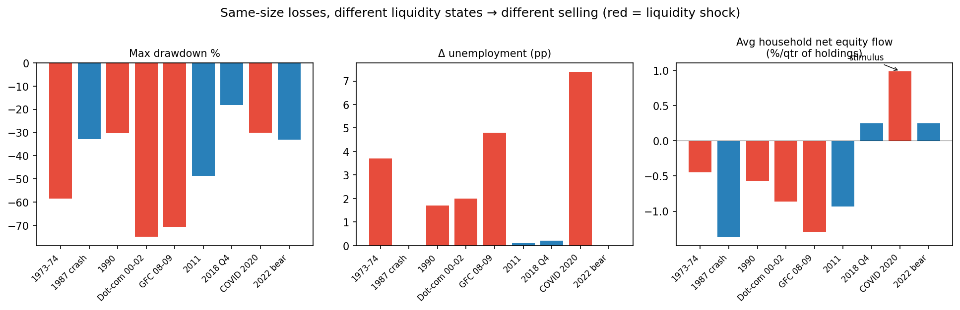
FRED and Federal Reserve Z.1 data: NASDAQ drawdowns, unemployment (urgency proxy), financial stress, retail money-market assets, and household net purchases of corporate equities as a share of holdings, quarterly.

episode max dd Δ unemp avg household net equity flow 1973-74 (shock) -58% +3.7pp -0.45 %/qtr seller 1987 (margin) -33% +0.0pp -1.37 %/qtr seller (leverage = λ) 1990 (shock) -30% +1.7pp -0.57 %/qtr seller dot-com (shock) -75% +2.0pp -0.86 %/qtr seller GFC (shock) -71% +4.8pp -1.29 %/qtr heaviest seller 2011 (no shock) -49% +0.1pp -0.93 %/qtr seller 2018Q4 (no shock) -18% +0.2pp +0.25 %/qtr BUYER COVID (shock+T) -30% +7.4pp +0.99 %/qtr BUYER (transfers hit λ) 2022 (no shock) -33% +0.0pp +0.25 %/qtr BUYER regression, 130 qtrs: stress β = -0.26 (t = -2.5) controlling for return; return alone: weak. The constraint moves the selling, not the loss.

The two decisive cells: 2022 — a one-third drawdown with slack constraints, and households bought; 2020 — the largest income shock on record, and households still bought, because CARES transfers replaced the lost liquidity (saving rate +15pp). The one cycle in which policy hit λ directly is the one cycle without capitulation. 1987, the apparent counterexample, was margin-call selling — leverage is simply another channel through which λ binds.

Drawdowns, urgency shocks, and household net equity flows, 1971-2026 — Fig. 1 — Drawdowns, urgency shocks, and household net equity flows, 1971–2026. Red bands: bears with liquidity shocks; blue: bears without.

Same-size losses, different liquidity states, different selling — Fig. 2 — Same-size losses, different liquidity states → different selling.

In the frequency domain, household-flow and drawdown variance concentrates at ~16-year periods (the credit cycle), unemployment at ~8–10 (the business cycle), with almost no power at the high frequencies where a sentiment story would live. In the cycle band, unemployment leads household selling by roughly seven quarters — a buffer-depletion lag. Agents do not sell the day liquidity escapes; they sell when the buffer runs out. A preference story has no natural account of that lag; a constraint story predicts it. The cascade restates as a transfer function: A = 1/(1−ρ) is the loop gain of a positive-feedback amplifier that magnifies low frequencies most — which is why the variance sits where it sits.

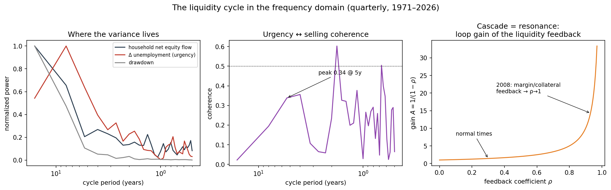
Fig. 3 — The liquidity cycle in the frequency domain. Left: variance concentrates at credit-cycle periods. Center: urgency–selling coherence. Right: cascade as resonance, gain 1/(1−ρ).

221 quarters contain roughly three realizations of a 16-year cycle; the spectrum is consistent with the theorem, not proof of it. Z.1 household flows are aggregate, buyback-distorted, and net forced sellers against dip buyers. The sharp identification remains the 2020/2022 pair.

§6 · Boundary conditions — what the literature already disproves

The strong version does not survive Genesove–Mayer (2001) runs exactly the identification this paper demands — the liquidity state (equity/LTV) observed — and loss aversion survives the control: Boston condo sellers facing nominal losses set asking prices 25–35% of the loss higher and sold slower, with equity constraints explaining under 20% of the variation. A Dutch administrative replication finds the nominal-loss effect roughly twice the negative-equity effect. Odean (1998) dismisses liquidity for brokerage sales (a cash-need seller sells anything; real sellers systematically pick winners); Weber–Camerer (1998) produce the disposition effect in the lab with no constraint in existence; Frazzini (2006) finds it in fund managers with no personal cash-need channel. The preference is real.

But note what that evidence concerns: the disposition margin — refusing to sell at a loss in normal times. It establishes the preference exists; it does not establish that crisis-wave selling is preference-driven, and the fire-sale literature points the other way on that margin. The findings compose rather than conflict: households hold losers until λ > 0 forces the sale. The preference governs the quiet regime; the constraint governs the loud one. The surviving theorem: crisis-state preference parameters are unidentified without λ, and pooled loss-aversion estimates are biased upward by its omission — coexistence with a bias term, not replacement.

§7 · What is missing from the literature

7.1 Genesove–Mayer in a crash

The benchmark identifies preferences in a regional, slow bust, on the listing margin. No study runs the same design inside a systemic capitulation window: a crisis-state decomposition of realized sales into contractual (stops, margin, redemptions), cash-need (λ > 0), and voluntary components, with the liquidity state observed. Scandinavian registry data — linked bank balances, unemployment-insurance records, security-level holdings — makes this feasible now; state-level UI generosity against 2008–09 U.S. brokerage records is the available quasi-experiment. This is the paper Theorem 1 says must exist, and it does not.

7.2 The contract share of forced supply

No unified measurement exists of what fraction of crisis volume is contractually forced — triggered stops, margin liquidations, redemption-driven fund sales (the Coval–Stafford channel) — versus discretionary. Broker order-type flags, FINRA margin statistics, and fund flows each capture a piece; nobody has assembled the decomposition Proposition 2 requires. Without it, ρ is not measurable ex ante, and neither is the distance to the cascade threshold.

7.3 The merged model

The behavioral literature estimates preferences without λ; the fire-sale literature models λ without preferences. A structural model in which reference-dependent agents choose the contracts that later force them — loss aversion as demand for stop-losses, stop-losses as supply of cascades — does not exist. Its comparative static is testable: markets with heavier retail stop-loss and margin penetration should exhibit larger A for identical fundamental shocks.

7.4 Past Piketty — a mechanism for r > g

The concentration ratchet as the pump behind the identity Piketty documents the accounting: when the return on wealth exceeds growth, wealth shares compound. But r > g is a description, not a mechanism — it does not say how the excess return is collected, by whom, or why it persists. The ratchet of §4 supplies the pump. The aggregate r is heterogeneous: r_permanent > r_constrained, and the spread is the urgency rent — the fire-sale discount collected each uninsured cycle, plus the foregone recovery on assets surrendered at the bottom. Concentration then advances step-wise, clustered at crises, not smoothly as the identity implies. Testable against Piketty: (i) top wealth-share gains should cluster in post-crisis recoveries (2009–2012 is one observation); (ii) cross-country concentration growth should scale with the number × amplitude of uninsured cycles, not merely average r−g; (iii) countries with stronger automatic liquidity stabilizers should show flatter ratchets holding tax policy fixed. The inversion: if the spread is a function of A, inequality dynamics are governed not only by taxation (Piketty's lever) but by liquidity insurance — compressing A compresses r−g at its source. Redistribution taxes the harvest; liquidity insurance prevents the harvesting.

7.5 The welfare accounting of the seed

No cost-benefit analysis treats eviction and foreclosure prevention as macro-stabilization rather than welfare policy. The object to be estimated is A itself: cascade losses prevented per dollar of bridge liquidity, inclusive of spillovers. The calibration above suggests order 10²; a defensible estimate would re-rank housing-stability spending against conventional stabilization tools.

§8 · Falsification

What would falsify the constraint channel: crisis-window micro data in which observed cash buffers, income shocks, and margin positions absorb none of the selling variance; or a liquidity instrument with zero effect on crisis selling. 2020 ran the reverse test and the channel passed. What would falsify the preference channel: Genesove–Mayer-style controls eliminating loss-aversion effects — already run, and the preference passed. Both channels are real; the open question is the decomposition, and §7.1–7.2 name the data that would settle it.

Empirical constants are pre-2025 literature ballparks flagged for verification before formal citation. References to be formalized: Kahneman–Tversky 1979; Shleifer–Vishny 1992; Odean 1998; Weber–Camerer 1998; Genesove–Mayer 2001; Kőszegi–Rabin 2006; Frazzini 2006; Coval–Stafford 2007; Brunnermeier–Pedersen 2009; Campbell–Giglio–Pathak 2011; Ben-David–Hirshleifer 2012; Desmond 2016; Piketty 2014. Data: FRED, Federal Reserve Z.1. Nothing herein is investment or legal advice.

← Book 6 index WP-31: The Calibration Pipeline →